Spiral Arms and CSST Project

December 2025

W51·December 21

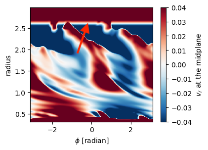
More problems

Another example of things going wrong. This times, likely some problem in the implementation of planet potential. Also, the movement of the planet in the azimuthal direction also means I am not calculating the planet position correctly to apply its gravity.

W50·December 12

Boundary problems

Above is an example of things going wrong. The straight line slightly beyond implies a circle in the Cartesian coordinates. The velocities with opposite signs on the two sides means gas is moving away from that circle on both sides which would produce a vacuum at that location. In other words, this is a good example of boundary conditions being not set correctly.

The steps to debug and sort out the problem are same as I’m already familiar with. Start with simple and most basic reduced form of the actual problem. Gradually add complexity, one at a time. See how things change.

W50·December 11

Leaky Gaps

Rixin Li has kindly hosted a tutorial on how to run hydro models with Athena++ at his webpage. This includes instructions to run/compile the code, as well as how to setup problem generators and even provides additional scripts to analyze, process and visualize the simulation data in a better way.

W49·December 5

A writeup

The first step is to setup the problem generator file. For our problem, we need to define following interface functions manually:

// This routine does two things: first is to read/parse the accompanying input file 
// and then enroll our custom defined source function (which in our case is the 
// planet-disk interaction) and BCs.
void Mesh::InitUserMeshData(ParameterInput *pin)
 
// This will be the core function that will setup the ICs.
void MeshBlock::ProblemGenerator(ParameterInput *pin)

Initial conditions

First step, is to setup the density which is given by:

where . I assumed , as that seems logical given we are using code units. For , we need to enforce the constraint that the total disk mass yields (although in code units might not be necessary?). I used , given seems obvious from figures (1-4) of the paper as well, written explicitly for the SPH simulation. Further, as planet is supposed to be at mid-plane, . For sound speed, we can use the fact that they use vertically isothermal disk, so

Now, we know,

we can use the temperature profile to find :

They chose such that:

which means

And, I think to get the final expression for , we can absorb the value of the constant factor in code units again, which gives us . Finally, we can also get an expression for aspect ratio:

Source function

This sets the ICs. Next, we need to set up the planet-disk source function. In the athena++ wiki, this is the place where we can update the conserved variables at each time step, like momentum and energy, but because we are using isothermal EOS, we need to worry only about momentum.

void MySource(MeshBlock *pmb, const Real time, const Real dt,
		const AthenaArray<Real> &prim,
		const AthenaArray<Real> &prim_scalar,
		const AthenaArray<Real> &bcc,
		AthenaArray<Real> &cons,
		AthenaArray<Real> &cons_scalar);

As I understand, for our case, I can just update the momentum by using the momentum density:

where and is given by equation (4) in the paper. Under our code units, , so I can just use the planetary mass at that instant to get the potential. As density is not going to change with time (except from fluxes), that term goes away. Finally,

Boundary conditions

From what I understand, for the radial direction, the authors have adopted symmetric BC, which I think athena++ calls reflective. But instead of reversing sign, they use damping zones, which I think is similar to outflow BC. So I am not sure which one to use. I implemented the damping zones in the source function itself.

For meridional direction, we need to implement a custom BC, as given by equation (9) of the paper:

Now, we can integrate from active cell to ghost cell:

For thin disk approximation, is small, so . Initially, , and from paper’s equation (3), varies as as we move away from mid-plane. With , we get . Therefore, for small , overall, also does not change much. In which case, we can simplify the integral as:

Note I use the values of active cell as we are integrating from active to ghost cell and is small, with respect to, . Integration of is trivial, which gives:

And for the azimuthal direction, I think periodic BC over the whole domain makes sense. For traversing the cells, I referred to the athena++ wiki page on BCs.

Azimuthal velocity in case of FARGO

In orbital advection runs, that is with FARGO enabled, the written to the output files is azimuthally averaged background velocity subtracted value. Let us calculate this azimuthally averaged background velocity. From Rixin’s notes accompanying the plotting notebook, the background velocity is given by:

A small note

The exoALMA paper also did not specify what order of orbital advection (FARGO) they used, so not sure which to use.

W49·December 3

Baseline

The work of (Bergez-Casalou et al., 2022) forms one of our baselines. The thing to keep in mind is images of the Solar System’s natal protoplanetary disk. We don’t deal with dust-gas dynamics, just gas dynamics. And instead of looking in the ALMA range of mm/sub-mm, we are going to look in optical/infrared. This is perhaps the right time to introduce Xuntian, or the Chinese space station survey telescope (CSST), the telescope that we will be targeting.

W49·December 2

Small jobs

When testing setups, especially for hydro models, it’s always nice to test with smaller resolution models. They are faster to solve!

W49·December 1

The exoALMA data

The data provided by (Bae et al., 2025) is available on the web. A good starting point was to obviously see if I can at least recreate the plots from the paper, from the paper’s data.

November 2025

W48·November 29

Project start

Setting up Athena++ on my local machine and familiarizing myself with the usual workflow. The official wiki hosted on GitHub is actually the best resource for getting accustomed to the codebase. But of course, for any meaningful simulations, one needs a distributed HPC cluster. Working with HPC means to learn how to submit and run jobs on a system whose resources are shared simultaneously by many. Resources for those:

1. A bit on sbatch
2. A bit on job scheduling
3. A bit on storage policies

In the end, each cluster might have their own set of policies. Always refer to the documentation!